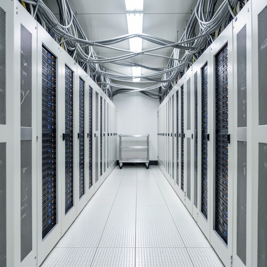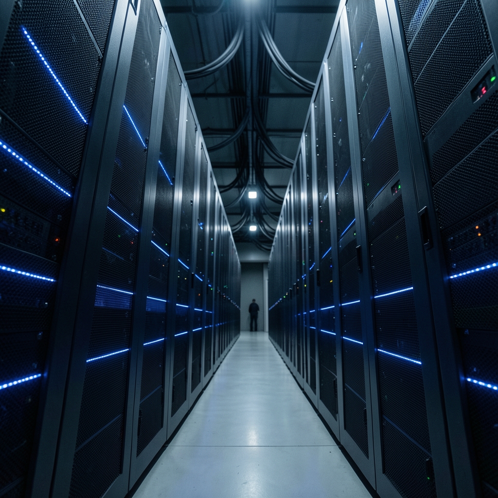
What happens between the moment someone clicks “run report” and the moment a chart appears on screen? Somewhere in that gap, a cloud data warehouse decides how to split the work, where to store the data, and how much compute to spend on the answer. Those decisions are not magic. They are architecture, and understanding them changes how teams design, budget, and troubleshoot their analytics. (AI cloud architecture: When infrastructure becomes intelligent)
This article walks through the core building blocks of a modern cloud data warehouse: separated storage and compute, columnar engines, massively parallel processing, open table formats, workload isolation, and the cost controls that keep everything honest.
Why storage and compute were split apart
For decades, data warehouses were appliances. Storage and processing power lived in the same box, so buying more disk meant paying for processors you did not need, and running a heavy month-end report could starve the dashboards everyone else was using.
Cloud warehouses broke that link. In the model described in Snowflake’s documentation on key concepts, data sits in cheap, durable object storage while virtual warehouses (independent compute clusters) read it on demand. You can pause compute when nobody is querying, resize it for a big transformation job, and scale storage without touching either.
The practical consequences are bigger than they sound:
- Elasticity: compute spins up in seconds and shuts down just as fast, so batch jobs no longer dictate cluster sizing for the whole month.
- Cost granularity: you pay for storage and compute on separate meters, which makes it possible to see that a dashboard refresh, not the data itself, is driving the bill.
- Failure isolation: a runaway query can be killed without taking the storage layer down with it.
The trade-off is that data now crosses a network between storage and compute. That is why cloud egress and data transfer charges deserve their own line in any architecture review, and a clearer way to track cloud data transfer costs can stop surprises before they land on an invoice.
Columnar storage and vectorized execution

Traditional row-store databases were built for transactions: fetch one customer record, update one order. Analytics asks the opposite question: scan a billion rows, sum one column. Reading whole rows to answer that is wasteful.
Cloud warehouses store data column by column. Each column holds values of the same type, which compresses well and lets the engine read only the columns a query touches. A query that sums revenue by region never loads the customer address column at all.
Amazon Redshift’s architecture documentation describes this columnar, massively parallel design in detail. The same idea appears in nearly every analytic engine, from BigQuery to DuckDB. Two performance habits follow directly from it: (BigQuery overview)
- Select only the columns you need. `SELECT *` on a wide table defeats the storage layout.
- Sort or cluster on the columns you filter most. Sorted data lets the engine skip whole blocks of rows, a technique usually called zone maps or min-max pruning.
Massively parallel processing, explained plainly
MPP, or massively parallel processing, means one query is split across many nodes that work at the same time. Each node holds a slice of the data. The query planner sends fragments of work to each slice, then combines the results.
The tricky part is data distribution. When two large tables are joined on a column, rows that need to meet must physically land on the same node. If the tables are distributed differently, the engine shuffles data across the network mid-query, a step often called redistribution. Redshift’s guidance on distribution and sort keys explains how choosing a distribution key that matches common join columns avoids that shuffle.
A useful mental model: MPP is a kitchen brigade. Each cook has a station. If a dish needs ingredients from three stations, someone has to carry them across the room. Good data modeling keeps ingredients near the station that needs them.
| Design choice | What it affects | Common mistake |
|---|---|---|
| Distribution key | Join performance, data skew | Picking a low-cardinality column, so one node gets most rows |
| Sort key | Range filtering, compression | Sorting on a column nobody filters by |
| Partitioning | Pruning on date or region | Partitioning too finely, creating tiny files |
| Clustering | Skipping irrelevant data | Clustering on a column with random values |
Serverless compute and the disappearing cluster
Not every warehouse asks you to size a cluster. Google BigQuery’s introduction describes a serverless model: you submit SQL, and the service allocates compute behind the scenes, billed either per query scanned or through reserved capacity measured in slots.
Serverless shifts the operational burden but not the design burden. You no longer tune node counts, yet you still control how much data each query scans. Partitioning, clustering, and avoiding repeated full-table scans matter just as much, arguably more, because the bill tracks bytes read rather than hours of cluster time.
Teams migrating between models often underestimate this. The inventory work before a cloud migration should include query patterns and table sizes in addition to schemas, because a query that was cheap on a fixed cluster can be expensive when priced per byte.
Open table formats and the lakehouse idea
For years, data lakes held files and data warehouses held tables, and the two worlds barely spoke. Open table formats changed that. Apache Iceberg, Delta Lake, and Apache Hudi add a metadata layer on top of files in object storage, providing ACID transactions, schema evolution, and time travel. The Apache Iceberg documentation covers these capabilities in depth.
The result is the lakehouse: warehouse-style management over lake-style cheap storage. The term was popularized in a research paper by Armbrust, Ghodsi, Xin, and Zaharia, which argued that the two architectures had converged and that a single system could serve BI, data science, and machine learning.
In practice, a lakehouse architecture usually means:
- One copy of data in open formats, readable by many engines.
- ACID guarantees so concurrent writers do not corrupt tables.
- Time travel for auditing and reproducible experiments.
- Governance applied at the table layer rather than per tool.
This convergence is a big part of why cloud infrastructure and architecture decisions now center on interoperability. Picking a warehouse that can read open formats reduces the risk of lock-in, though it does not eliminate it: query engines still differ in cost, SQL dialect, and performance characteristics.
Workload isolation: keeping dashboards fast during load
A single warehouse serving ingestion, transformation, and BI at once invites contention. The standard fix is to separate workloads onto distinct compute clusters. Snowflake’s multi-cluster warehouse documentation describes how additional clusters start automatically when queued queries pile up, then shut down when demand falls.
The pattern that works in practice:
- Loading cluster for ingestion, sized for steady throughput.
- Transformation cluster for scheduled dbt or SQL jobs, sized for bursts.
- BI cluster for dashboards, kept small but always available.
- Ad hoc cluster for analysts, with a query timeout and a spending cap.
The fourth one matters more than people expect. A single exploratory query joining two enormous tables can consume more compute than a month of dashboards. Giving analysts their own cluster with guardrails protects everyone else.
Security and governance inside the warehouse
Governance used to be bolted on: extract data, mask it in a separate tool, hope the copy is not left lying around. Modern warehouses push controls down to the data layer itself. Column-level security, row-level access policies, dynamic masking, and object tagging are now standard features, documented in Snowflake’s column-level security guide.
Three practices separate mature deployments from messy ones:
- Tag data at creation. Classification applied later rarely catches everything.
- Grant roles, not users. Role hierarchies survive staff turnover; individual grants do not.
- Test policies with real queries. A masking policy that breaks a dashboard gets removed within a week.
Enterprise AI and cloud security concerns amplify this. When a language model queries a warehouse on a user’s behalf, the model must inherit that user’s row-level permissions, not a service account’s. The same principle appears in separating tenant data in an enterprise assistant: isolation has to be enforced where the data lives, not where the chat window is.
Cost governance as an architectural feature
Because compute is metered, cost is a design property. Warehouses expose resource monitors, query history, and chargeback views precisely because spending can drift without anyone noticing. Redshift’s workload management documentation shows how query queues and concurrency scaling settings shape both performance and spend.
What actually works, based on common practice:
- Set resource monitors with hard stops, in addition to alerts. Alerts get ignored during a launch week.
- Review the top twenty queries by cost weekly. A small number usually dominates.
- Auto-suspend idle compute aggressively. A cluster idling overnight is pure waste.
- Attribute cost to teams. Chargeback changes behavior faster than any memo.
AI cloud architecture adds a new wrinkle: model training and inference jobs can generate unpredictable query volumes. Budgeting for those requires the same discipline as any other workload, plus a way to cap them.
How to read a vendor architecture announcement
Cloud vendors announce new regions, engines, and features constantly, and the announcements blend genuine capability with marketing. A useful habit is to separate three questions: what changed technically, what it costs, and what it replaces. A guide to reading a cloud region announcement walks through that filter, and the same lens applies to warehouse feature launches.
Vendor documentation is often technically accurate and promotional at the same time. Performance claims should be read as vendor-stated until an independent benchmark or your own workload confirms them. The honest test is always the same: run your queries on your data.
Conclusion
Cloud data warehouse architecture comes down to a handful of ideas that reinforce each other. Separating storage from compute makes elasticity possible. Columnar storage and MPP make large scans fast. Open table formats loosen the grip of any single vendor. Workload isolation keeps one team’s query from ruining another’s afternoon. Governance and cost controls turn all of that capability into something an organization can actually operate.
None of it runs itself. The teams that get the most from these systems are the ones that treat distribution keys, partitioning, permissions, and budgets as first-class design decisions rather than afterthoughts. Get those right, and the warehouse quietly does its job: turning a click into an answer, at a price nobody has to apologize for.
Frequently asked questions
What is the difference between a data lake and a cloud data warehouse?
A data lake stores raw files in object storage with minimal structure, which suits machine learning and unstructured data. A cloud data warehouse stores structured tables with schemas, transactions, and a query engine optimized for SQL analytics. Lakehouse architectures combine both by putting warehouse-style management, including ACID transactions and schema enforcement, on top of lake storage using open table formats.
Does separating storage and compute make queries slower?
It can add latency, because data must travel over a network between storage and compute. Well-designed engines compensate with caching, local disk staging, and metadata pruning that skips irrelevant files. For most analytical workloads the elasticity gained outweighs the transfer overhead, but teams should measure cold-start query times rather than assume parity with a tightly coupled system.
What does massively parallel processing actually do?
MPP splits a single query into fragments and runs them simultaneously across many nodes, each holding a slice of the data. The engine then combines partial results. Performance depends heavily on how data is distributed: joins on mismatched distribution keys trigger data shuffling across the network, which is often the real reason a query is slow.
Do I still need to tune a serverless warehouse?
Yes, though the knobs differ. With serverless engines you do not size clusters, but you still control how many bytes each query scans. Partitioning tables by date, clustering on frequently filtered columns, and avoiding repeated full-table scans directly reduce cost. A poorly partitioned table can cost many times more than a well-designed one on identical hardware.
How do I stop one team’s queries from slowing everyone else down?
Give each workload its own compute cluster: separate ones for loading, transformation, business intelligence, and ad hoc analysis. Add query timeouts and spending limits to the ad hoc cluster, since exploratory queries are the most unpredictable. This isolation pattern is standard in cloud warehouses and is usually cheaper than buying one oversized cluster for everyone.
Are open table formats ready for production?
They are widely used in production, particularly Iceberg and Delta Lake, and they provide ACID transactions, schema evolution, and time travel over object storage. The caveats are operational: small-file problems accumulate without compaction, catalog choices matter, and engine support for the newest features varies. Teams should test their specific query patterns before migrating critical tables.